Improve Your Circuit Manufacturing Yield With Monte Carlo Analysis In PSpice! (Part 4 of 4)
To begin with this blog, it's important to be clear on what exactly does -Manufacturing Yield mean? Formally, the definition of Yield states: 
Circuit Maufacturing Yield:
Here's a simple graphical- way to understand the meaning of-Circuit Yield, refer-to Figure 1 (below)
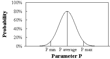
Figure 1: Simple Yield Diagram of any Circuit
The-above Yield Figure shows-that the circuit will work-between the limits Pmin and Pmax with an approximate yield of a little less than 100%. Also,-note that yield is -best in the region around P average -when probability is the highest.
Why is such a Yield graph helpful for any circuit?
Importance:

It is astonishing that today a circuit designer can quantify failures before beginning mass manufacturing of the boards.
Let's understand the importance with two more examples- If you are producing large quantity of PCB boards, you would worry about even 0.1% rejection. When building mission critical project for Military/ Space application, you cannot afford to have your design fail in any scenario. Thus, you would keep minimal/ no variation of components in your design. Monte Carlo comes to your rescue in such situations! With Yield prediction, you can evaluate if tighter component tolerances (at a higher cost) will be better for your product/ design. Else, lower tolerance components can save you a lot of money.
Would you not like to achieve 100% yield? Be sure that your design is "truly" ready for mass production. Monte Carlo statistically predicts behavior of any circuit for a set of varied component values within their tolerance range. It calculates yield and presents-it in an easy to understand graphical format (like Figure 4), so you can balance yield and cost.-
Let's look at the easy steps required to perform Monte Carlo Analysis in PSpice,
Flow For Monte Carlo Analysis:

Circuit Used For Monte Carlo Analysis:
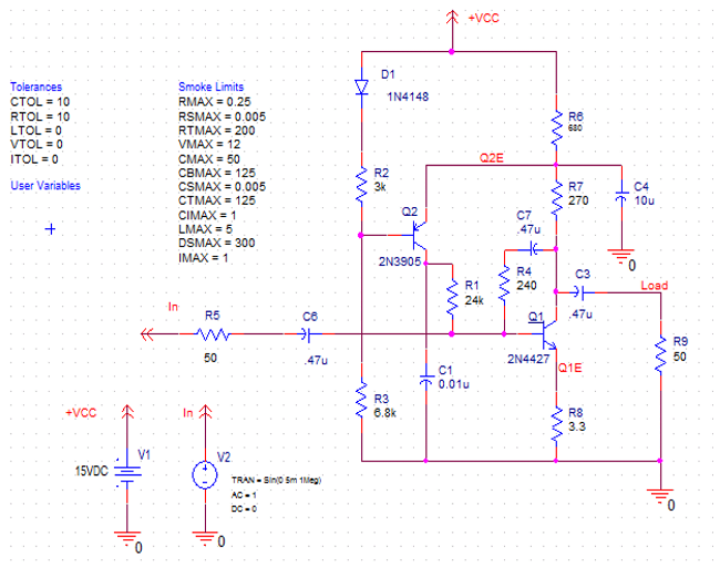
Figure 2: RF Amplifier Circuit
The design shown in Figure 2 (above) is- same as the one we used in Blog 3 -(on Smoke Analysis)- after Transistor Replacement. Going back to the steps required for performing Monte Carlo Analysis, we have already assigned the Tolerances and set the Measurement expressions in- Blog 1-(on Sensitivity Analysis). All we have to do is run Monte Carlo Analysis on this design after giving appropriate values as shown in Profile Settings tab below (Figure 3)
Running Monte Carlo Analysis (Profile Settings):
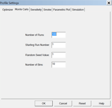
Figure 3: Profile settings required before running Monte Carlo Analysis
Understanding Setting Options:
- Number of Runs: This is the number of times the selected simulation profiles will be run. For each run, component parameters with tolerances will be randomly varied. More the simulation runs, more accurate the yield prediction. Better the yield, more the profit margin!
- Starting Run number: The default starting run number is one. This is the nominal run.
- Random Seed Value: The random number generator uses this value to produce a sequence of random numbers for Monte Carlo Simulation
- Number of Bins: This value determines the number of divisions in the histogram
Monte Carlo calculates a nominal value for each measurement using the original parameter values. After the nominal runs, algorithm randomly calculates the value of each variable parameter based on its tolerance with a flat (uniform) distribution or a Gaussian distribution function. For each profile, it uses the calculated parameter values, evaluates the measurements, and saves those values.-
After running Monte Carlo analysis on this design, the output window-looks like- Figure 4-(below)
Monte Carlo Output Environment:
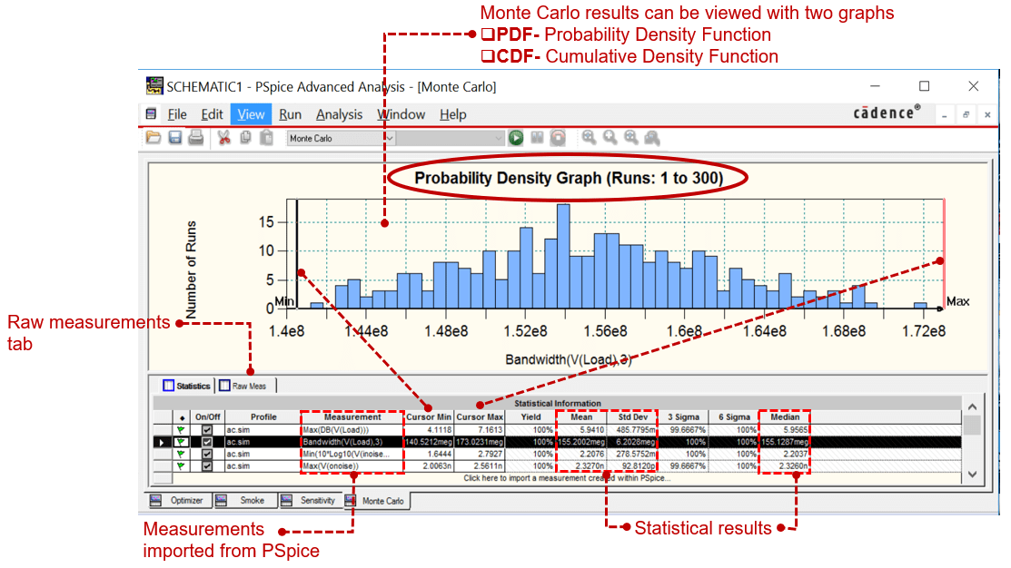
Figure 4: Output window after performing Monte Carlo Analysis
The graph above displays -the range of measurement values along the X-axis and the number of runs with those measurement values along the Y-axis. Probability Distribution can be displayed in either-Probability Distribution Function (PDF) or Cumulative Distribution Function (CDF) graph.
Note, that the measurements are the same we used in Using Sensitivity Analysis In PSpice, Grab A Coffee And Let Optimizer In PSpice Do The Work For You! and Use Smoke Analysis In PSpice; of Gain, Bandwidth, Noise Figure and Output Noise. Monte Carlo Analysis calculated the yield for each of these measurements varying the tolerance range of each component in the circuit, thus giving a holistic realization any circuit's capability.
For this circuit, the selected Bandwidth measurement in Figure 4 shows that the Yield is 100% for the entire frequency range from 0.14 GHz to 0.17 GHz. Same applies for the other three measurement values. It simply means that all our goals are met with perfection within the specified frequency range which is great!
Generic SPICE Technology vs PSpice AA Technology:
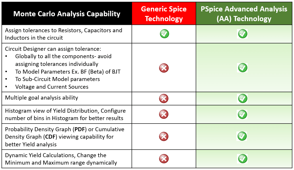
Let's wrap this Tech Blog series with a value proposition for each PSpice Advanced Analysis capability that we have,
Figure 5: Overall PSpice Advanced Analysis Capabilities
Thus, you can leverage PSpice Advanced Analysis to reduce design cost, improve design reliability, engineer's productivity and manufacturing yield.
Utilize Monte Carlo Analysis within PSpice Advanced Analysis to increase the Yield of any circuit design.
Refer to the other 3 blogs of this series here,
1. Know How Your Circuit Works!- Using Sensitivity Analysis In PSpice (Part 1 of 4)
2. Grab A Coffee And Let Optimizer In PSpice Do The Work For You! (Part 2 of 4)
3. Make Reliable Designs That Won’t Fail In The Real World!- Use Smoke Analysis In PSpice (Part 3 of 4)
Video reference: Leverage PSpice Advanced Analysis to reduce design cost, improve design reliability, engineer's productivity and manufacturing yield.
Try the OrCAD X free trial yourself and start applying these Advanced Analysis capabilities on one of the many demo designs available in there.